Wednesday, September 30, 2020

Store and Access Time Series Data at Any Scale with Amazon Timestream – Now Generally Available

Time series are a very common data format that describes how things change over time. Some of the most common sources are industrial machines and IoT devices, IT infrastructure stacks (such as hardware, software, and networking components), and applications that share their results over time. Managing time series data efficiently is not easy because the data model doesn’t fit general-purpose databases.

For this reason, I am happy to share that Amazon Timestream is now generally available. Timestream is a fast, scalable, and serverless time series database service that makes it easy to collect, store, and process trillions of time series events per day up to 1,000 times faster and at as little as to 1/10th the cost of a relational database.

This is made possible by the way Timestream is managing data: recent data is kept in memory and historical data is moved to cost-optimized storage based on a retention policy you define. All data is always automatically replicated across multiple availability zones (AZ) in the same AWS region. New data is written to the memory store, where data is replicated across three AZs before returning success of the operation. Data replication is quorum based such that the loss of nodes, or an entire AZ, does not disrupt durability or availability. In addition, data in the memory store is continuously backed up to Amazon Simple Storage Service (S3) as an extra precaution.

Queries automatically access and combine recent and historical data across tiers without the need to specify the storage location, and support time series-specific functionalities to help you identify trends and patterns in data in near real time.

There are no upfront costs, you pay only for the data you write, store, or query. Based on the load, Timestream automatically scales up or down to adjust capacity, without the need to manage the underlying infrastructure.

Timestream integrates with popular services for data collection, visualization, and machine learning, making it easy to use with existing and new applications. For example, you can ingest data directly from AWS IoT Core, Amazon Kinesis Data Analytics for Apache Flink, AWS IoT Greengrass, and Amazon MSK. You can visualize data stored in Timestream from Amazon QuickSight, and use Amazon SageMaker to apply machine learning algorithms to time series data, for example for anomaly detection. You can use Timestream fine-grained AWS Identity and Access Management (IAM) permissions to easily ingest or query data from an AWS Lambda function. We are providing the tools to use Timestream with open source platforms such as Apache Kafka, Telegraf, Prometheus, and Grafana.

Using Amazon Timestream from the Console
In the Timestream console, I select Create database. I can choose to create a Standard database or a Sample database populated with sample data. I proceed with a standard database and I name it MyDatabase.

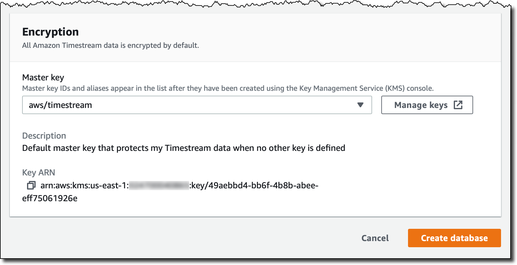
All Timestream data is encrypted by default. I use the default master key, but you can use a customer managed key that you created using AWS Key Management Service (KMS). In that way, you can control the rotation of the master key, and who has permissions to use or manage it.

I complete the creation of the database. Now my database is empty. I select Create table and name it MyTable.

Each table has its own data retention policy. First data is ingested in the memory store, where it can be stored from a minimum of one hour to a maximum of a year. After that, it is automatically moved to the magnetic store, where it can be kept up from a minimum of one day to a maximum of 200 years, after which it is deleted. In my case, I select 1 hour of memory store retention and 5 years of magnetic store retention.

When writing data in Timestream, you cannot insert data that is older than the retention period of the memory store. For example, in my case I will not be able to insert records older than 1 hour. Similarly, you cannot insert data with a future timestamp.

I complete the creation of the table. As you noticed, I was not asked for a data schema. Timestream will automatically infer that as data is ingested. Now, let’s put some data in the table!

Loading Data in Amazon Timestream
Each record in a Timestream table is a single data point in the time series and contains:

  • The measure name, type, and value. Each record can contain a single measure, but different measure names and types can be stored in the same table.
  • The timestamp of when the measure was collected, with nanosecond granularity.
  • Zero or more dimensions that describe the measure and can be used to filter or aggregate data. Records in a table can have different dimensions.

For example, let’s build a simple monitoring application collecting CPU, memory, swap, and disk usage from a server. Each server is identified by a hostname and has a location expressed as a country and a city.

In this case, the dimensions would be the same for all records:

  • country
  • city
  • hostname

Records in the table are going to measure different things. The measure names I use are:

  • cpu_utilization
  • memory_utilization
  • swap_utilization
  • disk_utilization

Measure type is DOUBLE for all of them.

For the monitoring application, I am using Python. To collect monitoring information I use the psutil module that I can install with:

pip3 install plutil

Here’s the code for the collect.py application:

import time
import boto3
import psutil

from botocore.config import Config

DATABASE_NAME = "MyDatabase"
TABLE_NAME = "MyTable"

COUNTRY = "UK"
CITY = "London"
HOSTNAME = "MyHostname" # You can make it dynamic using socket.gethostname()

INTERVAL = 1 # Seconds

def prepare_record(measure_name, measure_value):
    record = {
        'Time': str(current_time),
        'Dimensions': dimensions,
        'MeasureName': measure_name,
        'MeasureValue': str(measure_value),
        'MeasureValueType': 'DOUBLE'
    }
    return record


def write_records(records):
    try:
        result = write_client.write_records(DatabaseName=DATABASE_NAME,
                                            TableName=TABLE_NAME,
                                            Records=records,
                                            CommonAttributes={})
        status = result['ResponseMetadata']['HTTPStatusCode']
        print("Processed %d records. WriteRecords Status: %s" %
              (len(records), status))
    except Exception as err:
        print("Error:", err)


if __name__ == '__main__':

    session = boto3.Session()
    write_client = session.client('timestream-write', config=Config(
        read_timeout=20, max_pool_connections=5000, retries={'max_attempts': 10}))
    query_client = session.client('timestream-query')

    dimensions = [
        {'Name': 'country', 'Value': COUNTRY},
        {'Name': 'city', 'Value': CITY},
        {'Name': 'hostname', 'Value': HOSTNAME},
    ]

    records = []

    while True:

        current_time = int(time.time() * 1000)
        cpu_utilization = psutil.cpu_percent()
        memory_utilization = psutil.virtual_memory().percent
        swap_utilization = psutil.swap_memory().percent
        disk_utilization = psutil.disk_usage('/').percent

        records.append(prepare_record('cpu_utilization', cpu_utilization))
        records.append(prepare_record(
            'memory_utilization', memory_utilization))
        records.append(prepare_record('swap_utilization', swap_utilization))
        records.append(prepare_record('disk_utilization', disk_utilization))

        print("records {} - cpu {} - memory {} - swap {} - disk {}".format(
            len(records), cpu_utilization, memory_utilization,
            swap_utilization, disk_utilization))

        if len(records) == 100:
            write_records(records)
            records = []

        time.sleep(INTERVAL)

I start the collect.py application. Every 100 records, data is written in the MyData table:

$ python3 collect.py
records 4 - cpu 31.6 - memory 65.3 - swap 73.8 - disk 5.7
records 8 - cpu 18.3 - memory 64.9 - swap 73.8 - disk 5.7
records 12 - cpu 15.1 - memory 64.8 - swap 73.8 - disk 5.7
. . .
records 96 - cpu 44.1 - memory 64.2 - swap 73.8 - disk 5.7
records 100 - cpu 46.8 - memory 64.1 - swap 73.8 - disk 5.7
Processed 100 records. WriteRecords Status: 200
records 4 - cpu 36.3 - memory 64.1 - swap 73.8 - disk 5.7
records 8 - cpu 31.7 - memory 64.1 - swap 73.8 - disk 5.7
records 12 - cpu 38.8 - memory 64.1 - swap 73.8 - disk 5.7
. . .

Now, in the Timestream console, I see the schema of the MyData table, automatically updated based on the data ingested:

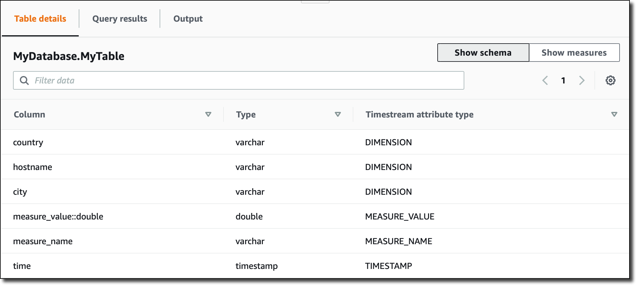
Note that, since all measures in the table are of type DOUBLE, the measure_value::double column contains the value for all of them. If the measures were of different types (for example, INT or BIGINT) I would have more columns (such as measure_value::int and measure_value::bigint) .

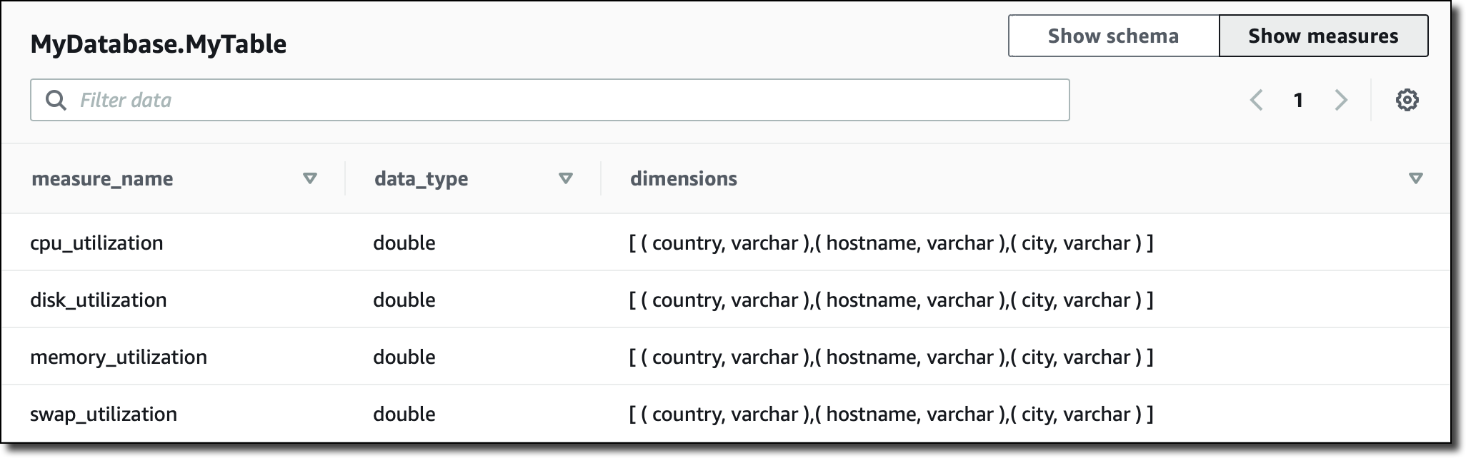
In the console, I can also see a recap of which kind measures I have in the table, their corresponding data type, and the dimensions used for that specific measure:

Querying Data from the Console
I can query time series data using SQL. The memory store is optimized for fast point-in-time queries, while the magnetic store is optimized for fast analytical queries. However, queries automatically process data on all stores (memory and magnetic) without having to specify the data location in the query.

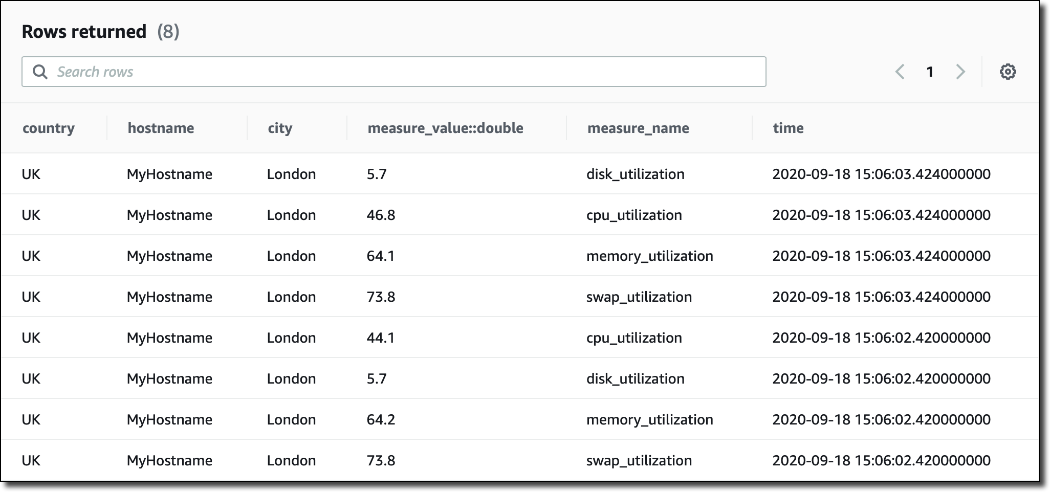
I am running queries straight from the console, but I can also use JDBC connectivity to access the query engine. I start with a basic query to see the most recent records in the table:

SELECT * FROM MyDatabase.MyTable ORDER BY time DESC LIMIT 8

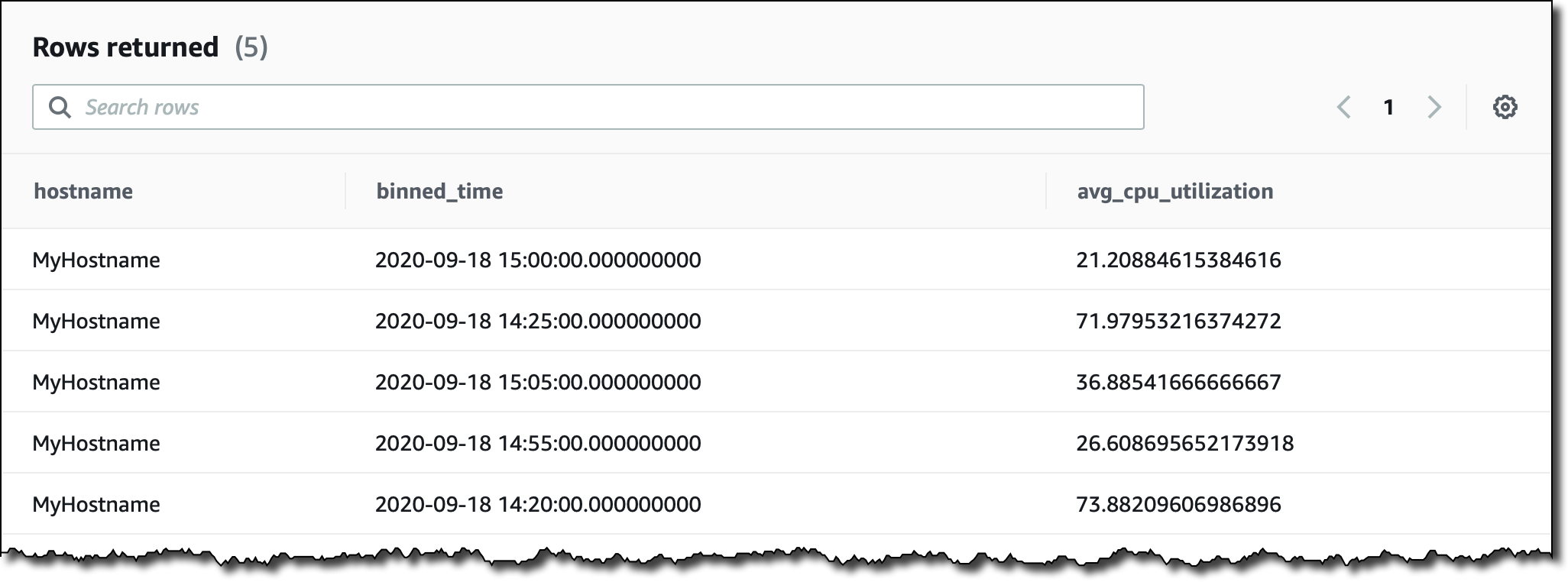
Let’s try something a little more complex. I want to see the average CPU utilization aggregated by hostname in 5 minutes intervals for the last two hours. I filter records based on the content of measure_name. I use the function bin() to round time to a multiple of an interval size, and the function ago() to compare timestamps:

SELECT hostname,
       bin(time, 5m) as binned_time,
       avg(measure_value::double) as avg_cpu_utilization
  FROM MyDatabase.MyTable
 WHERE measure_name = ‘cpu_utilization'
   AND time > ago(2h)
 GROUP BY hostname, bin(time, 5m)

When collecting time series data you may miss some values. This is quite common especially for distributed architectures and IoT devices. Timestream has some interesting functions that you can use to fill in the missing values, for example using linear interpolation, or based on the last observation carried forward.

More generally, Timestream offers many functions that help you to use mathematical expressions, manipulate strings, arrays, and date/time values, use regular expressions, and work with aggregations/windows.

To experience what you can do with Timestream, you can create a sample database and add the two IoT and DevOps datasets that we provide. Then, in the console query interface, look at the sample queries to get a glimpse of some of the more advanced functionalities:

Using Amazon Timestream with Grafana
One of the most interesting aspects of Timestream is the integration with many platforms. For example, you can visualize your time series data and create alerts using Grafana 7.1 or higher. The Timestream plugin is part of the open source edition of Grafana.

I add a new GrafanaDemo table to my database, and use another sample application to continuously ingest data. The application simulates performance data collected from a microservice architecture running on thousands of hosts.

I install Grafana on an Amazon Elastic Compute Cloud (EC2) instance and add the Timestream plugin using the Grafana CLI.

$ grafana-cli plugins install grafana-timestream-datasource

I use SSH Port Forwarding to access the Grafana console from my laptop:

$ ssh -L 3000:<EC2-Public-DNS>:3000 -N -f ec2-user@<EC2-Public-DNS>

In the Grafana console, I configure the plugin with the right AWS credentials, and the Timestream database and table. Now, I can select the sample dashboard, distributed as part of the Timestream plugin, using data from the GrafanaDemo table where performance data is continuously collected:

Available Now
Amazon Timestream is available today in US East (N. Virginia), Europe (Ireland), US West (Oregon), and US East (Ohio). You can use Timestream with the console, the AWS Command Line Interface (CLI), AWS SDKs, and AWS CloudFormation. With Timestream, you pay based on the number of writes, the data scanned by the queries, and the storage used. For more information, please see the pricing page.

You can find more sample applications in this repo. To learn more, please see the documentation. It’s never been easier to work with time series, including data ingestion, retention, access, and storage tiering. Let me know what you are going to build!

Danilo

Via AWS News Blog https://ift.tt/1EusYcK

Amazon S3 on Outposts Now Available

AWS Outposts customers can now use Amazon Simple Storage Service (S3) APIs to store and retrieve data in the same way they would access or use data in a regular AWS Region. This means that many tools, apps, scripts, or utilities that already use S3 APIs, either directly or through SDKs, can now be configured to store that data locally on your Outposts.

AWS Outposts are a fully managed service that provides a consistent hybrid experience, with AWS installing the Outpost in your data center or colo facility. These Outposts are managed, monitored, and updated by AWS just like in the cloud. Customers use AWS Outposts to run services in their local environments, like Amazon Elastic Compute Cloud (EC2), Amazon Elastic Block Store (EBS), and Amazon Relational Database Service (RDS), and are ideal for workloads that require low latency access to on-premises systems, local data processing, or local data storage.

Outposts are connected to an AWS Region and are also able to access Amazon S3 in AWS Regions, however, this new feature will allow you to use the S3 APIs to store data on the AWS Outposts hardware and process it locally. You can use S3 on Outposts to satisfy demanding performance needs by keeping data close to on-premises applications. It will also benefit you if you want to reduce data transfers to AWS Regions, since you can perform filtering, compression, or other pre-processing on your data locally without having to send all of it to a region.

Speaking of keeping your data local, any objects and the associated metadata and tags are always stored on the Outpost and are never sent or stored elsewhere. However, it is essential to remember that if you have data residency requirements, you may need to put some guardrails in place to ensure no one has the permissions to copy objects manually from your Outposts to an AWS Region.

You can create S3 buckets on your Outpost and easily store and retrieve objects using the same Console, APIs, and SDKs that you would use in a regular AWS Region. Using the S3 APIs and features, S3 on Outposts makes it easy to store, secure, tag, retrieve, report on, and control access to the data on your Outpost.

S3 on Outposts provides a new Amazon S3 storage class, named S3 Outposts, which uses the S3 APIs, and is designed to durably and redundantly store data across multiple devices and servers on your Outposts. By default, all data stored is encrypted using server-side encryption with SSE-S3. You can optionally use server-side encryption with your own encryption keys (SSE-C) by specifying an encryption key as part of your object API requests.

When configuring your Outpost you can add 48 TB or 96 TB of S3 storage capacity, and you can create up to 100 buckets on each Outpost. If you have existing Outposts, you can add capacity via the AWS Outposts Console or speak to your AWS account team. If you are using no more than 11 TB of EBS storage on an existing Outpost today you can add up to 48 TB with no hardware changes on the existing Outposts. Other configurations will require additional hardware on the Outpost (if the hardware footprint supports this) in order to add S3 storage.

So let me show you how I can create an S3 bucket on my Outposts and then store and retrieve some data in that bucket.

Storing data using S3 on Outposts

To get started, I updated my AWS Command Line Interface (CLI) to the latest version. I can create a new Bucket with the following command and specify which outpost I would like the bucket created on by using the –outposts-id switch.

aws s3control create-bucket --bucket my-news-blog-bucket --outposts-id op-12345

In response to the command, I am given the ARN of the bucket. I take note of this as I will need it in the next command.

Next, I will create an Access point. Access points are a relatively new way to manage access to an S3 bucket. Each access point enforces distinct permissions and network controls for any request made through it. S3 on Outposts requires a Amazon Virtual Private Cloud configuration so I need to provide the VPC details along with the create-access-point command.

aws s3control create-access-point --account-id 12345 --name prod --bucket "arn:aws:s3-outposts:us-west-2:12345:outpost/op-12345/bucket/my-news-blog-bucket" --vpc-configuration VpcId=vpc-12345

S3 on Outposts uses endpoints to connect to Outposts buckets so that you can perform actions within your virtual private cloud (VPC). To create an endpoint, I run the following command.

aws s3outposts create-endpoint --outpost-id op-12345 --subnet-id subnet-12345 —security-group-id sg-12345

Now that I have set things up, I can start storing data. I use the put-object command to store an object in my newly created Amazon Simple Storage Service (S3) bucket.

aws s3api put-object --key my_news_blog_archives.zip --body my_news_blog_archives.zip --bucket arn:aws:s3-outposts:us-west-2:12345:outpost/op-12345/accesspoint/prod

Once the object is stored I can retrieve it by using the get-object command.

aws s3api get-object --key my_news_blog_archives.zip --bucket arn:aws:s3-outposts:us-west-2:12345:outpost/op-12345/accesspoint/prod my_news_blog_archives.zip

There we have it. I’ve managed to store an object and then retrieve it, on my Outposts, using S3 on Outposts.

Transferring Data from Outposts

Now that you can store and retrieve data on your Outposts, you might want to transfer results to S3 in an AWS Region, or transfer data from AWS Regions to your Outposts for frequent local access, processing, and storage. You can use AWS DataSync to do this with the newly launched support for S3 on Outposts.

With DataSync, you can choose which objects to transfer, when to transfer them, and how much network bandwidth to use. DataSync also encrypts your data in-transit, verifies data integrity in-transit and at-rest, and provides granular visibility into the transfer process through Amazon CloudWatch metrics, logs, and events.

Order today

If you want to start using S3 on Outposts, please visit the AWS Outposts Console, here you can add S3 storage to your existing Outposts or order an Outposts configuration that includes the desired amount of S3. If you’d like to discuss your Outposts purchase in more detail then contact our sales team.

Pricing with AWS Outposts works a little bit differently from most AWS services, in that it is not a pay-as-you-go service. You purchase Outposts capacity for a 3-year term and you can choose from a number of different payment schedules. There are a variety of AWS Outposts configurations featuring a combination of EC2 instance types and storage options. You can also increase your EC2 and storage capacity over time by upgrading your configuration. For more detailed information about pricing check out the AWS Outposts Pricing details.

Happy Storing

— Martin Via AWS News Blog https://ift.tt/1EusYcK

Tuesday, September 29, 2020

2 egregious cloud security threats the CSA missed

My interesting weekend reading was this Cloud Security Alliance (CSA) report, which was vendor sponsored, highlighting 11 cloud security threats that should be on top of everyone’s mind. These threats are described as “egregious.”

CSA surveyed 241 experts on security issues in the cloud industry and came up with these top 11 threats:

  1. Data breaches
  2. Misconfiguration and inadequate change control
  3. Lack of cloud security architecture and strategy
  4. Insufficient identity, credential, access, and key management
  5. Account hijacking
  6. Insider threat
  7. Insecure interfaces and APIs
  8. Weak control plane
  9. Metastructure and applistructure failures
  10. Limited cloud usage visibility
  11. Abuse and nefarious use of cloud services

This is a pretty good report, by the way. It’s free to download, and if you’re interested in the evolution of cloud computing security, it’s a good read.  

To read this article in full, please click here

Friday, September 25, 2020

When AIops tools outsmart you

Our ability to augment technology with artificial intelligence and machine learning does not seem to have limits. We now have AI-powered analytics, smart Internet of Things, AI at the edge, and of course AIops tools.

At their essence, AIops tools do smart automations. These include self-healing, proactive maintenance, even working with security and governance systems to coordinate actions, such as identifying a performance issue as a breach.

We need to consider discovery as well, or the capability of gathering data ongoing and leveraging that data to train the knowledge engine. This allows the knowledgebases to become savvier. Greater knowledge about how the systems under management behave or are likely to behave creates a better capability of predicting issues and being proactive around fixes and reporting. 

To read this article in full, please click here

Tuesday, September 22, 2020

Will cloud architecture change after COVID?

A few things have changed since the start of the COVID-19 lockdowns. The Global 2000, as well as governments, now understand that traditional data centers are more vulnerable to natural disasters (such as pandemics) than once thought.  

Indeed, the use of cloud computing means that there are no physical data centers and servers to protect, and that we don’t rely on humans for physical operations as much as we did in the past.  

Putting the obvious aside for now, let’s look at the future of cloud computing, specifically at the future of cloud computing architecture. I see a few changes happening now that won’t likely go away after the current crisis ends:

To read this article in full, please click here

Friday, September 18, 2020

When a digital twin becomes the evil twin

A digital twin is a digital replica of some physical entity, such as a person, a device, manufacturing equipment, or even planes and cars. The idea is to provide a real-time simulation of a physical asset or human to determine when problems are likely to occur and to proactively fix them before they actually arise.

Although the roles of digital twins vary a great deal, the connection is established using real-time data from sensors that are able to sync the digital twin living in a virtual world with the physical twin that we can actually touch. This new synchronized simulation leverages IoT (Internet of Things), AI (artificial intelligence), machine learning, and analytics with spatial graphics to create a working simulation of the model that updates as the physical entity changes. 

To read this article in full, please click here

Tuesday, September 15, 2020

Amazon Transcribe Now Supports Automatic Language Identification

In 2017, we launched Amazon Transcribe, an automatic speech recognition service that makes it easy for developers to add a speech-to-text capability to their applications. Since then, we added support for more languages, enabling customers globally to transcribe audio recordings in 31 languages, including 6 in real-time.

A popular use case for Amazon Transcribe is transcribing customer calls. This allows companies to analyze the transcribed text using natural language processing techniques to detect sentiment or to identify the most common call causes. If you operate in a country with multiple official languages or across multiple regions, your audio files can contain different languages. Thus, files have to be tagged manually with the appropriate language before transcription can take place. This typically involves setting up teams of multi-lingual speakers, which creates additional costs and delays in processing audio files.

The media and entertainment industry often uses Amazon Transcribe to convert media content into accessible and searchable text files. Use cases include generating subtitles or transcripts, moderating content, and more. Amazon Transcribe is also used by operations team for quality control, for example checking that audio and video are in sync thanks to the timestamps present in the extracted text. However, other problems couldn’t be easily solved, such as verifying that the main spoken language in your videos is correctly labeled to avoid streaming video in the wrong language.

Today, I’m extremely happy to announce that Amazon Transcribe can now automatically identify the dominant language in an audio recording. This feature will help customers build more efficient transcription workflows by getting rid of manual tagging. In addition to the examples mentioned above, you can now also easily use Amazon Transcribe to automatically recognize and transcribe voicemails, meetings, and any form of recorded communication.

Introducing Automatic Language Identification
With a minimum of 30 seconds of audio, Amazon Transcribe can efficiently generate transcripts in the spoken language without wasting time and resources on manual tagging. Automatic identification of the dominant language is available in batch transcription mode for all 31 languages. Thanks to sampling techniques, language identification happens much faster than the transcription itself, in the matter of seconds.

If you’re already using Amazon Transcribe for speech recognition, you just need to enable the feature in the StartTranscriptionJob API. Before your transcription job is complete, the response of the GetTranscriptionJob API will tell the dominant language of the audio recording, and its confidence score between 0 and 1. The transcript lists the top five languages and their respective confidence scores.

Of course, if you want to use Amazon Transcribe exclusively for automatic language identification, you can simply process the API response and ignore the transcript. In this case, you should stick to short 30-45 second audio recordings to minimize costs.

You can also restrict languages that Amazon Transcribe tries to identify, by passing a list of languages to the StartTranscriptionJob API. For example, if your company call center only receives calls in English, Spanish and French, then restricting identifiable languages to this list will increase language identification accuracy.

Now, I’d like to show you how easy it us to use this new feature!

Detecting the Dominant Language With Amazon Transcribe
First, let’s try a high quality sample. I’ll use the audio track from one of my breakout sessions at AWS Summit Paris 2019. I can easily download it using the youtube-dl tool.

$ youtube-dl -f bestaudio https://www.youtube.com/watch?v=AFN5jaTurfA
$ mv AWS\ \&\ EarthCube\ _\ Deep\ learning\ démarrer\ avec\ MXNet\ et\ Tensorflow\ en\ 10\ minutes-AFN5jaTurfA.m4a video.m4a

Using ffmpeg, I shorten the audio clip to 1 minute.

$ ffmpeg -i video.m4a -ss 00:00:00.00 -t 00:01:00.00 video-1mn.m4a

Then, I upload the clip to an Amazon Simple Storage Service (S3) bucket.

$ aws s3 cp video-1mn.m4a s3://jsimon-transcribe-uswest2/

Next, I use the AWS CLI to run a transcription job on this audio clip, with language identification enabled.

$ awscli transcribe start-transcription-job --transcription-job-name video-test --identify-language --media MediaFileUri=s3://jsimon-transcribe-uswest2/video-1mn.m4a

Waiting only a few seconds, I check the status of the job. I could also use a Amazon CloudWatch event to be notified that language identification is complete.

$ awscli transcribe get-transcription-job --transcription-job-name video-test
{
    "TranscriptionJob": {
        "TranscriptionJobName": "video-test",
        "TranscriptionJobStatus": "IN_PROGRESS",
        "LanguageCode": "fr-FR",
        "MediaSampleRateHertz": 44100,
        "MediaFormat": "mp4",
        "Media": {
        "MediaFileUri": "s3://jsimon-transcribe-uswest2/video-1mn.m4a"
    },
    "Transcript": {},
    "StartTime": 1593704323.312,
"CreationTime": 1593704323.287,

    "Settings": {
        "ChannelIdentification": false,
        "ShowAlternatives": false
    },
    "IdentifyLanguage": true,
    "IdentifiedLanguageScore": 0.915885329246521
    }
}

As highlighted in the output, the dominant language has been correctly detected in seconds, with a high confidence score of 91.59%. A few more seconds later, the transcription job is complete. Running the same CLI call, I can retrieve a link to the transcription, which also includes the top 5 languages for the audio clip, sorted by decreasing score.

"language_identification":[{"score":"0.9159","code":"fr-FR"},{"score":"0.0839","code":"fr-CA"},{"score":"0.0001","code":"en-GB"},{"score":"0.0001","code":"pt-PT"},{"score":"0.0001","code":"de-CH"}]

Adding up French and Canadian French, we pretty much get a score of 100%, so there’s no doubt that this clip is in French. In some cases, you may not care for that level of detail, and you’ll see in the next example how to restrict the list of detected languages.

Restricting the List of Detected Languages
As customer call transcription is a popular use case for Amazon Transcribe, here is a 40-second audio clip (WAV, 8KHz, 16-bit resolution), where I’m reading a paragraph from the French version of the Amazon Transcribe page. As you can hear, quality is pretty awful, and I added background music (Bach-ground, actually) for good measure.

Again, I upload the clip to an S3 bucket, and I use the AWS CLI to transcribe it. This time, I restrict the list of languages to French, Spanish, German, US English, and British English.

$ aws s3 cp speech-8k.wav s3://jsimon-transcribe-uswest2/
$ awscli transcribe start-transcription-job --transcription-job-name speech-8k-test --identify-language --media MediaFileUri=s3://jsimon-transcribe-uswest2/speech-8k.wav --language-options fr-FR es-ES de-DE en-US en-GB

A few seconds later, I check the status of the job.

$ awscli transcribe get-transcription-job --transcription-job-name speech-8k-test
{
    "TranscriptionJob": {
    "TranscriptionJobName": "speech-8k-test",
    "TranscriptionJobStatus": "IN_PROGRESS",
    "LanguageCode": "fr-FR",
    "MediaSampleRateHertz": 8000,
    "MediaFormat": "wav",
    "Media": {
        "MediaFileUri": "s3://jsimon-transcribe-uswest2/speech-8k.wav"
    },
    "Transcript": {},
    "StartTime": 1593705151.446,
"CreationTime": 1593705151.423,

    "Settings": {
        "ChannelIdentification": false,
        "ShowAlternatives": false
    },
    "IdentifyLanguage": true,
    "LanguageOptions": [
        "fr-FR","es-ES","de-DE","en-US","en-GB"
    ],
    "IdentifiedLanguageScore": 0.9995
    }
}

As highlighted in the output, the dominant language has been correctly detected with a very high confidence score in spite of the terrible audio quality. Restricting the list of languages certainly helps, and you should use it whenever possible.

Getting Started
Automatic Language Identification is available today in these regions:

  • US East (N. Virginia), US East (Ohio), US West (N. California), US West (Oregon), AWS GovCloud (US-West).
  • Canada (Central).
  • South America (São Paulo).
  • Europe (Ireland), Europe (London), Europe (Paris), Europe (Frankfurt).
  • Middle East (Bahrain).
  • Asia Pacific (Hong Kong), Asia Pacific (Mumbai), Asia Pacific (Tokyo), Asia Pacific (Seoul), Asia Pacific (Singapore), Asia Pacific (Sydney).

There is no additional charge on top of the existing pricing. Give it a try, and please send us feedback either through your usual AWS Support contacts, or on the AWS Forum for Amazon Transcribe.

- Julien Via AWS News Blog https://ift.tt/1EusYcK

Rethinking 'cloud bursting'

About two years ago I wrote a piece here on the concept of cloud bursting, where I pointed out a few realities:

  • Private clouds are no longer a thing, considering the current state of private cloud systems compared to the features and functions of the larger hyperscalers.
  • You need to maintain workloads on both private and public clouds for hybrid cloud bursting to work; in essence, using two different platforms.
  • It’s clear the bursting hybrid clouds concept just adds too much complexity and cost for a technology stack (the cloud) to be widely adopted by companies that want to do the most with the least.

In case you missed the fervor in the tech press a few years ago, cloud bursting is the concept of leveraging public clouds only when capacity of the on-premises cloud runs out. Somehow companies thought that they could invoke a public cloud-based part of the application and have access to the same data without latency. Mostly it did not work.

To read this article in full, please click here

Monday, September 14, 2020

New EC2 T4g Instances – Burstable Performance Powered by AWS Graviton2 – Try Them for Free

Two years ago Amazon Elastic Compute Cloud (EC2) T3 instances were first made available, offering a very cost effective way to run general purpose workloads. While current T3 instances offer sufficient compute performance for many use cases, many customers have told us that they have additional workloads that would benefit from increased peak performance and lower cost.

Today, we are launching T4g instances, a new generation of low cost burstable instance type powered by AWS Graviton2, a processor custom built by AWS using 64-bit Arm Neoverse cores. Using T4g instances you can enjoy a performance benefit of up to 40% at a 20% lower cost in comparison to T3 instances, providing the best price/performance for a broader spectrum of workloads.

T4g instances are designed for applications that don’t use CPU at full power most of the time, using the same credit model as T3 instances with unlimited mode enabled by default. Examples of production workloads that require high CPU performance only during times of heavy data processing are web/application servers, small/medium data stores, and many microservices. Compared to previous generations, the performance of T4g instances makes it possible to migrate additional workloads such as caching servers, search engine indexing, and e-commerce platforms.

T4g instances are available in 7 sizes providing up to 5 Gbps of network and up to 2.7 Gbps of Amazon Elastic Block Store (EBS) performance:

Name vCPUs Baseline Performance/vCPU CPU Credits Earned/Hour Memory
t4g.nano 2 5% 6 0.5 GiB
t4g.micro 2 10% 12 1 GiB
t4g.small 2 20% 24 2 GiB
t4g.medium 2 20% 24 4 GiB
t4g.large 2 30% 36 8 GiB
t4g.xlarge 4 40% 96 16 GiB
t4g.2xlarge 8 40% 192 32 GiB

Free Trial
To make it easier to develop, test, and run your applications on T4g instances, all AWS customers are automatically enrolled in a free trial on the t4g.micro size. Starting September 2020 until December 31st 2020, you can run a t4g.micro instance and automatically get 750 free hours per month deducted from your bill, including any CPU credits during the free 750 hours of usage. The 750 hours are calculated in aggregate across all regions. For details on terms and conditions of the free trial, please refer to the EC2 FAQs.

During the free trial, have a look at this getting started guide on using the Arm-based AWS Graviton processors. There, you can find suggestions on how to build and optimize your applications, using different programming languages and operating systems, and on managing container-based workloads. Some of the tips are specific for the Graviton processor, but most of the content works generally for anyone using Arm to run their code.

Using T4g Instances
You can start an EC2 instance in different ways, for example using the EC2 console, the AWS Command Line Interface (CLI), AWS SDKs, or AWS CloudFormation. For my first T4g instance, I use the AWS CLI:

$ aws ec2 run-instances \
  --instance-type t4g.micro \
  --image-id ami-09a67037138f86e67 \
  --security-groups MySecurityGroup \
  --key-name my-key-pair

The Amazon Machine Image (AMI) I am using is based on Amazon Linux 2. Other platforms are available, such as Ubuntu 18.04 or newer, Red Hat Enterprise Linux 8.0 and newer, and SUSE Enterprise Server 15 and newer. You can find additional AMIs in the AWS Marketplace, for example Fedora, Debian, NetBSD, CentOS, and NGINX Plus. For containerized applications, Amazon ECS and Amazon Elastic Kubernetes Service optimized AMIs are available as well.

The security group I selected gives me SSH access to the instance. I connect to the instance and do a general update:

$ sudo yum update -y

Since the kernel has been updated, I reboot the instance.

I’d like to set up this instance as a development environment. I can use it to build new applications, or to recompile my existing apps to the 64-bit Arm architecture. To install most development tools, such as Git, GCC, and Make, I use this group of packages:

$ sudo yum groupinstall -y "Development Tools"

AWS is working with several open source communities to drive improvements to the performance of software stacks running on AWS Graviton2. For example, you can see our contributions to PHP for Arm64 in this post.

Using the latest versions helps you obtain maximum performance from your Graviton2-based instances. The amazon-linux-extras command enables new versions for some of my favorite programming environments:

$ sudo amazon-linux-extras enable golang1.11 corretto8 php7.4 python3.8 ruby2.6

The output of the amazon-linux-extras command tells me which packages to install with yum:

$ yum clean metadata
$ sudo yum install -y golang java-1.8.0-amazon-corretto \
  php-cli php-pdo php-fpm php-json php-mysqlnd \
  python38 ruby ruby-irb rubygem-rake rubygem-json rubygems

Let’s check the versions of the tools that I just installed:

$ go version
go version go1.13.14 linux/arm64
$ java -version
openjdk version "1.8.0_265"
OpenJDK Runtime Environment Corretto-8.265.01.1 (build 1.8.0_265-b01)
OpenJDK 64-Bit Server VM Corretto-8.265.01.1 (build 25.265-b01, mixed mode)
$ php -v
PHP 7.4.9 (cli) (built: Aug 21 2020 21:45:13) ( NTS )
Copyright (c) The PHP Group
Zend Engine v3.4.0, Copyright (c) Zend Technologies
$ python3.8 -V
Python 3.8.5
$ ruby -v
ruby 2.6.3p62 (2019-04-16 revision 67580) [aarch64-linux]

It looks like I am ready to go! Many more packages are available with yum, such as MariaDB and PostgreSQL. If you’re interested in databases, you might also want to try the preview of Amazon RDS powered by AWS Graviton2 processors.

Available Now
T4g instances are available today in US East (N. Virginia, Ohio), US West (Oregon), Asia Pacific (Tokyo, Mumbai), Europe (Frankfurt, Ireland).

You now have a broad choice of Graviton2-based instances to better optimize your workloads for cost and performance: low cost burstable general-purpose (T4g), general purpose (M6g), compute optimized (C6g) and memory optimized (R6g) instances. Local NVMe-based SSD storage options are also available.

You can use the free trial to develop new applications, or migrate your existing workloads to the AWS Graviton2 processor. Let me know how that goes!

Danilo

Via AWS News Blog https://ift.tt/1EusYcK

Friday, September 11, 2020

As edge computing evolves, the cloud's role changes

The notion of edge computing typically conjures an image of a device in a factory someplace, providing rudimentary computing and data collection to support a piece of manufacturing equipment. Perhaps it keeps the factory temperature and humidity optimized for the manufacturing process.

Those who deal with edge computing these days understand that what was considered “edge” just a few years ago has morphed into something a bit more involved. Here are the emerging edge computing architecture patterns that I’m seeing:

The new edge hierarchy. No longer are edge devices connected directly to some centralized system, such as one residing in the cloud. They connect to other edge devices that may connect to larger edge devices that ultimately connect to a centralized system or cloud.

To read this article in full, please click here

Tuesday, September 8, 2020

Some observations on cloud computing observability

The term and the concept of observability aren't new at all. Observability first appeared in the world of engineering and control theory. Although the definition depends on whom you’re asking, some common patterns and understandings are emerging. Mostly it’s a new buzzword by the AIops providers and some thought leaders in the cloudops space (meaning me). 

At its essence, observability is the measure of how well internal system states can be inferred from knowledge of all external data and states. It’s a bit different than monitoring which is something you do (a verb); observability is an attribute of a system (a noun).

If that’s a bit confusing, here's a more pragmatic definition: the ability to leverage the concept of observability and the tools that support that concept. Most monitoring and operations tools (such as AIops tools) claim some role in observability. However in some respects, to me it's the same old bourbon (monitoring) in a much fancier bottle (observability). I look at it with a bit of well-placed skepticism.

To read this article in full, please click here

Friday, September 4, 2020

AWS Named as a Cloud Leader for the 10th Consecutive Year in Gartner’s Infrastructure & Platform Services Magic Quadrant

At AWS, we strive to provide you a technology platform that allows for agile development, rapid deployment, and unlimited scale, so that you can free up your resources to focus on innovation for your customers. It’s greatly rewarding to see our efforts recognized not just by our customers, but also by leading analysts.

This year, Gartner announced a new Magic Quadrant for Cloud Infrastructure and Platform Services (CIPS). This is an evolution of their Magic Quadrant for Cloud Infrastructure as a Service (IaaS) for which AWS has been named as a Leader for nine consecutive years.

Customers are using the cloud in broad ways, beyond foundational compute, networking and storage services. We believe for this reason, Gartner is expanding the scope to include additional platform as a service (PaaS) capabilities, and is extending coverage for areas such as managed database services, serverless computing, and developer tools.

Today, I am happy to share that AWS has been named as a Leader in the Magic Quadrant for Cloud Infrastructure and Platform Services, and placed highest in Ability to Execute and furthest in Completeness of Vision.

More information on the features and factors that our customers examine when choosing a cloud provider are available in the full report.

Danilo

Gartner, Magic Quadrant for Cloud Infrastructure and Platform Services, Raj Bala, Bob Gill, Dennis Smith, David Wright, Kevin Ji, 1 September 2020 – Gartner does not endorse any vendor, product or service depicted in its research publications, and does not advise technology users to select only those vendors with the highest ratings or other designation. Gartner research publications consist of the opinions of Gartner’s research organization and should not be construed as statements of fact. Gartner disclaims all warranties, expressed or implied, with respect to this research, including any warranties of merchantability or fitness for a particular purpose.
Via AWS News Blog https://ift.tt/1EusYcK

Higher ed needs a course in cloud computing

Four-year colleges may face up to a 20 percent reduction in fall enrollment, according to SimpsonScarborough, a higher education research and marketing company. Its findings are based on surveys of more than 2,000 college-bound high school seniors and current college students. 

According to the Chronicle of Higher Education, nine percent of institutions plan to operate only online during the fall semester. The remainder will take a hybrid approach, with some classes offered online, while other classes will operate both online and in-person. 

To read this article in full, please click here

Tuesday, September 1, 2020

Dealing with sovereign data in the cloud

It’s Friday, and you’re about to close your laptop and go to happy hour, when you get an urgent e-mail stating that due to data being illegally transported out of the country, the company has been fined $250,000.  

What happened?

As bad luck would have it, your cloud provider backs up the database containing sovereign data to a storage system outside of the country. This is done for a good reason: Relocating data for business continuity and disaster recovery purposes to another region reduces the risk of data loss if the primary region is down. 

To read this article in full, please click here